Karl D. Lerud, Ph.D.
Auditory perception: Stimulus design and analysis
Project maintained by lerud Hosted on GitHub Pages — Theme by mattgraham
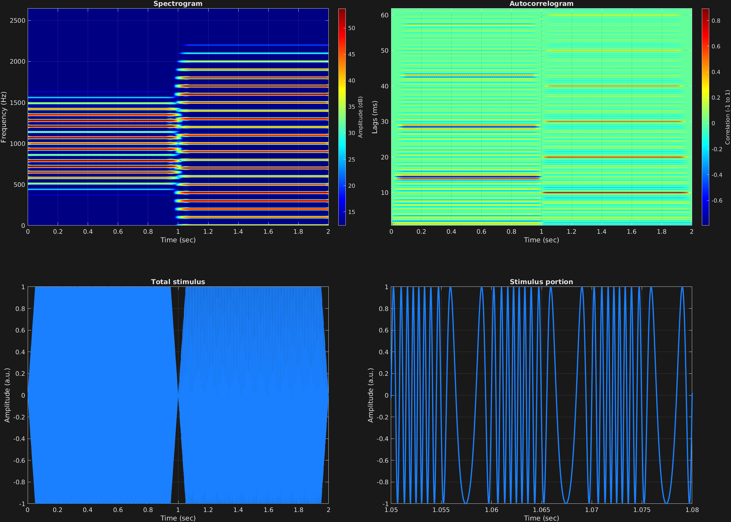
In this frequency modulation example, faster modulation is explored. As with amplitude modulation, when faster frequencies are used for modulation, predictable additions to the spectrum of the signal are observed as a function of the modulation frequencies and depths. Here we have two time spans, each with a different modulation frequency and depth. We remember the frequency modulation equation:
$$x(t)=a_c\sin \big(2\pi f_c t+a_m\sin(2\pi f_m t)+\theta_c\big)$$
In the latter time span, $f_c$ is an integer multiple of $f_m$, giving a harmonic spectrum with fundamental $f_0 =f_m =100$ Hz.
% Some plotting parameters
colorRatio=.67;
NFFT=8192*4;
specFreqPerc=[0 12];
specWindowLength=5000;
autoFreqPerc=[1 80];
xTimes=[1.05 1.08];

% Stimulus parameters
tSpans=[0 1;
        1 2];
fs=44100;
carWaves={'sin'};
carFreqs=1000;
carAmps=1;
carThs=0;
rampTime=.05;
rampExp=1;
fmFreq=[70;
        100];
fmAmp=[.35;
       .8];

% Create stimulus structure
s = stimulusMake(1, 'fcn', tSpans, fs, carWaves, carFreqs, carAmps, carThs, ...
    'ramp', rampTime, rampExp, 'fm', {'sin'}, fmFreq, fmAmp);

% Do some visualization
figure(1)
set(gcf,'position',[50 50 1700 1350])

subplot(2,2,1)
[~,~,cbar]=mdlSpec(s.x,NFFT,s.fs,specFreqPerc,specWindowLength);
grid on
temp=get(cbar,'limits');
colormap('jet')
totalRange=diff(temp);
cutoff=(colorRatio*totalRange)+temp(1);
caxis([cutoff temp(2)])

subplot(2,2,2)
mdlAutocorr(s.x,s.fs,autoFreqPerc);
grid on

subplot(2,2,3)
plot(s.t,s.x)
title('Total stimulus')
xlabel('Time (sec)')
ylabel('Amplitude (a.u.)')
grid on
zoom xon

subplot(2,2,4)
plot(s.t,s.x,'linewidth',2)
title('Stimulus portion')
xlabel('Time (sec)')
ylabel('Amplitude (a.u.)')
xlim(xTimes)
grid on
zoom xon