Karl D. Lerud, Ph.D.
Auditory perception: Stimulus design and analysis
Project maintained by lerud Hosted on GitHub Pages — Theme by mattgraham
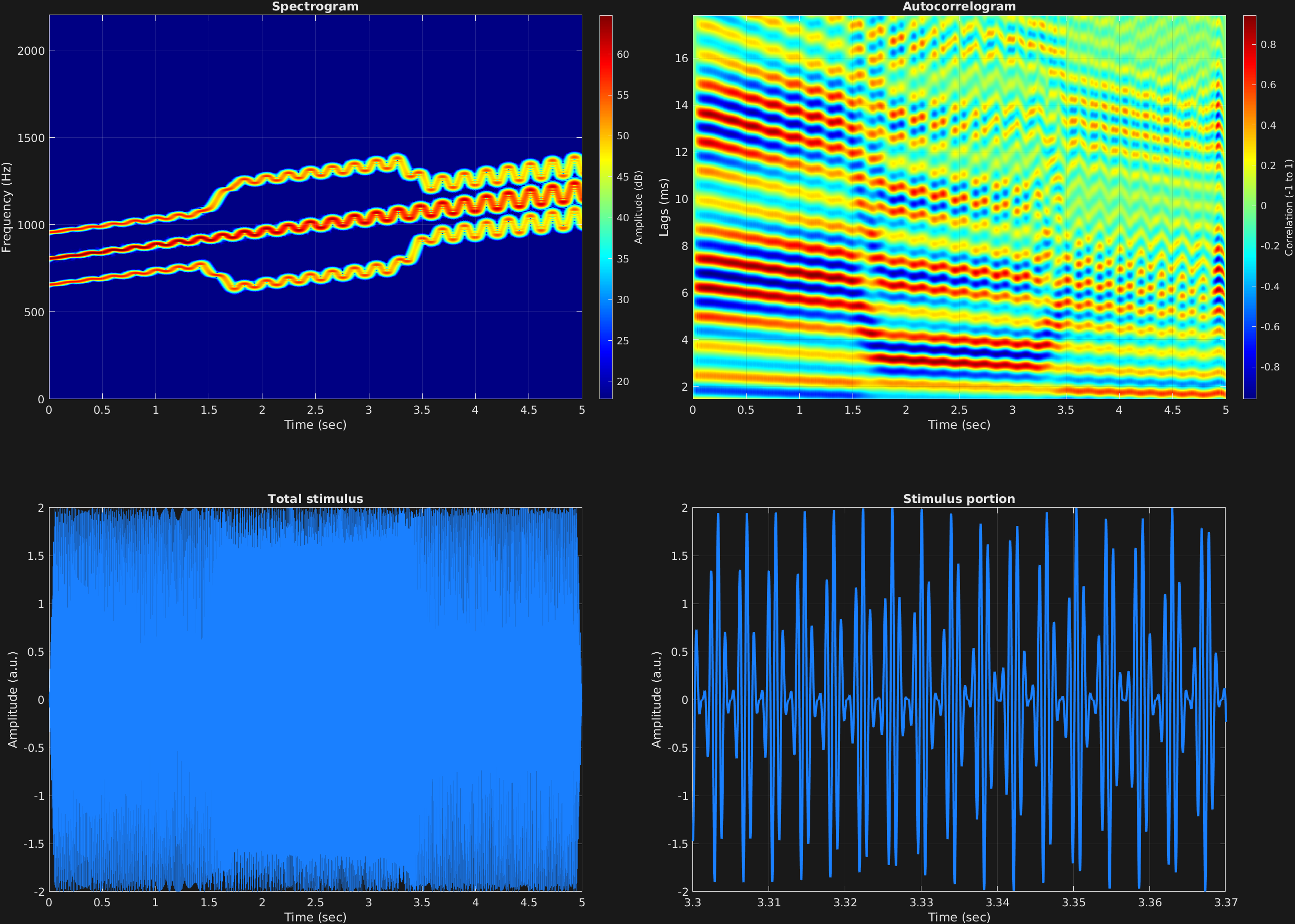
This example automates carrier frequency, amplitude modulation frequency, and frequency modulation amplitude. Firstly, the carrier frequency is slowly moving upward throughout. Secondly, the carrier is amplitude modulated throughout with a fast frequency, giving upper and lower sidebands which shift in the middle portion because of a change in amplitude modulation frequency. Thirdly, the carrier is frequency modulated with a slow frequency which is increasing in its depth throughout. The result of the latter is that all frequencies in the signal spectrum are frequency-modulated together.
% Some plotting parameters
colorRatio=.67;
NFFT=8192*4;
specFreqPerc=[0 10];
specWindowLength=7000;
autoFreqPerc=[1 12];
xTimes=[3.3 3.37];

% Stimulus parameters
tSpans=[0 5];
fs=44100;
carWaves={'sin'};
carFreqs={[800 1200]};
carAmps=1;
carThs=0;
rampTime=.05;
rampExp=1;
fmFreq=5;
fmAmp={[0 .05]};
amFreq={[ones(1,500)*150 linspace(150,300,100) ones(1,500)*300 linspace(300,150,100) ones(1,500)*150]};
amAmp=1;
amCfreq=1;

% Create stimulus structure
s = stimulusMake(1, 'fcn', tSpans, fs, {'sin'}, carFreqs, carAmps, 'ramp', rampTime, rampExp, ...
    'fm', {'sin'}, fmFreq, fmAmp, 'am', {'sin'}, amFreq, amAmp, amCfreq);


% Do some visualization
figure(1)
set(gcf,'position',[50 50 1700 1350])

subplot(2,2,1)
[~,~,cbar]=mdlSpec(s.x,NFFT,s.fs,specFreqPerc,specWindowLength);
grid on
temp=get(cbar,'limits');
colormap('jet')
totalRange=diff(temp);
cutoff=(colorRatio*totalRange)+temp(1);
caxis([cutoff temp(2)])

subplot(2,2,2)
mdlAutocorr(s.x,s.fs,autoFreqPerc);
grid on

subplot(2,2,3)
plot(s.t,s.x)
title('Total stimulus')
xlabel('Time (sec)')
ylabel('Amplitude (a.u.)')
grid on
zoom xon

subplot(2,2,4)
plot(s.t,s.x,'linewidth',2)
title('Stimulus portion')
xlabel('Time (sec)')
ylabel('Amplitude (a.u.)')
xlim(xTimes)
grid on
zoom xon
